Visualizing quadrature functions as point clouds#
Author: Henrik N.T. Finsberg
SPDX-License-Identifier: MIT
Quadrature functions are not possible to visualize directly in ParaView, as they are not defined on a mesh.
However, we can visualize them as point clouds.
In this example we will show how you can use scifem to save your quadrature functions as XDMF files,
which can be loaded into ParaView for visualization.
Note
This demo requires a backend for writing HDF5 files. Please install scifem with either scifem[adios2] or scifem[h5py].
First, we import the necessary modules.
# First initialize logging
logging.basicConfig(level=logging.INFO)
Now let’s create a quadrature function on a unit square mesh. We will use the basix.ufl module to create the quadrature element.
mesh = dolfinx.mesh.create_unit_square(MPI.COMM_WORLD, 10, 10, dolfinx.mesh.CellType.triangle, dtype=np.float64)
el = basix.ufl.quadrature_element(
    scheme="default", degree=3, cell=mesh.basix_cell(), value_shape=()
)
V = dolfinx.fem.functionspace(mesh, el)
u = dolfinx.fem.Function(V)
u.interpolate(lambda x: np.sin(np.pi * x[0]) * np.sin(np.pi * x[1]))
One option that already exists with the current DOLFINx/Pyvista API is to plot them as points
import pyvista
plotter = pyvista.Plotter()
plotter.add_points(
    V.tabulate_dof_coordinates(),
    scalars=u.x.array,
    render_points_as_spheres=True,
    point_size=20,
    show_scalar_bar=False,
)
plotter.export_vtksz("xdmf_point_cloud.vtksz")
plotter.show(screenshot="xdmf_point_cloud.png")
/tmp/ipykernel_997/289272519.py:9: PyVistaDeprecationWarning: Plotter.export_vtksz is deprecated. Use plotter.trame.export_vtksz(...) instead. Install via `pip install trame-pyvista`.
  plotter.export_vtksz("xdmf_point_cloud.vtksz")
INFO:trame_rca.encoders.image_encoder:Turbo JPEG - NOT AVAILABLE (Python package)
INFO:trame_rca.encoders:VTKStreaming Video encoding is NOT AVAILABLE (missing Python package)
INFO:trame_rca.schedulers:cannot import name 'RcaVideoEncoder' from 'trame_rca.encoders' (/dolfinx-env/lib/python3.14/site-packages/trame_rca/encoders/__init__.py)
INFO:trame_server.utils.namespace:Translator(prefix=None)
INFO:wslink.backends.aiohttp:awaiting runner setup
INFO:wslink.backends.aiohttp:awaiting site startup
INFO:wslink.backends.aiohttp:Print WSLINK_READY_MSG
INFO:wslink.backends.aiohttp:Schedule auto shutdown with timeout 0
INFO:wslink.backends.aiohttp:awaiting running future
Using scifem, we can write the point cloud data to an XDMFFile that can be opened with Paraview.
with scifem.xdmf.XDMFFile("point_cloud.xdmf", [u]) as xdmf:
    xdmf.write(0.0)
The point cloud can now be loaded into ParaView for visualization, by selecting “Point Gaussian” as the representation.
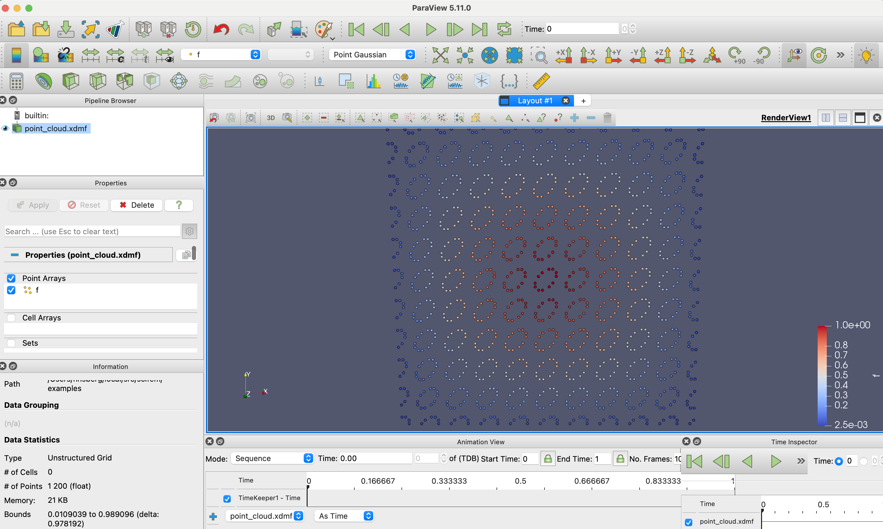
We can write any dolfinx.fem.FunctionSpace that has support for tabulate_dof_coordinates to a point cloud.
For example, we can create a higher order Lagrange space, and write two functions to file.
Q = dolfinx.fem.functionspace(mesh, ("Lagrange", 3, (2, )))
q_1 = dolfinx.fem.Function(Q, name="q_sin")
q_1.interpolate(lambda x: (np.sin(np.pi * x[0]),  np.sin(np.pi * x[1])))
q_2 = dolfinx.fem.Function(Q, name="q_cos")
q_2.interpolate(lambda x: (np.cos(np.pi * x[0]),  np.cos(np.pi * x[1])))
We write these two functions to file as illustrated above
with scifem.xdmf.XDMFFile("point_cloud_lagrange.xdmf", [q_1, q_2]) as xdmf:
    xdmf.write(0.0)
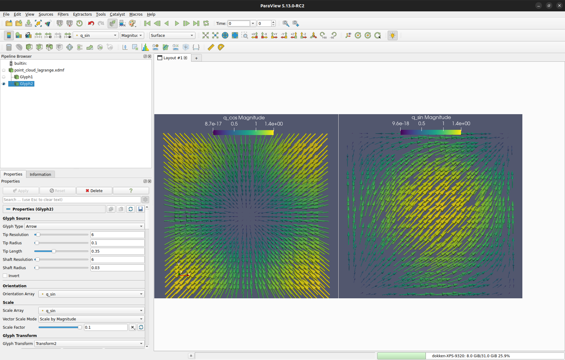
yielding the following point clouds in ParaView after applying glyphs.
If you have time dependent data, you can write multiple time steps to the same file using e.g
with scifem.xdmf.XDMFFile("point_cloud_lagrange.xdmf", [q_1, q_2]) as xdmf:
    xdmf.write(0.0)
    q_1.interpolate(lambda x: (-x[0], x[1]))
    q_2.interpolate(lambda x: (x[0], -x[1]))
    xdmf.write(0.3)
If you need to keep the file open for longer, you can use the following syntax
xdmf = scifem.xdmf.XDMFFile("point_cloud_lagrange.xdmf", [q_1, q_2])
xdmf.write(0.0)
q_1.interpolate(lambda x: (-x[0], x[1]))
q_2.interpolate(lambda x: (x[0], -x[1]))
xdmf.write(0.3)
xdmf.close()