Topology Optimization of a Linear-Elastic Cantilever (SIMP)

Section author: Jørgen S. Dokken (dokken@simula.no).

This demo reproduces the 3D cantilever-beam topology optimization problem from Pasteur Labs’ Mosaic benchmark suite, using dolfinx_adjoint in place of the original FEniCS/dolfin-adjoint solver. The mesh, material model, boundary conditions and objective follow Mosaic’s own reference implementation.

The optimizer differs from Mosaic’s own Adam-based recipe: this demo uses scipy.optimize.minimize(method="trust-constr"), driven by a pyadjoint.ReducedFunctionalNumPy, which unlike Mosaic’s Adam + manual clipping, enforces the SIMP density bounds natively via bounds= while also using exact Hessian-vector products from the adjoint/tangent-linear system (hessp=).

The per-iteration density animation uses the pyvista GIF-writing pattern from dolfinx-tutorial/chapter2/amr.py.

Problem definition

We minimize the structural compliance \(C = \mathbf{F}^\top \mathbf{u}\) of a linear elastic body \(\Omega\) subject to

\[\begin{split} \begin{align} -\operatorname{div}(\sigma(\mathbf u)) &= 0 &&\text{in } \Omega,\\ \mathbf{u} &= 0 && \text{on } \Gamma_D, \\ \sigma(\mathbf u)\cdot n &= \mathbf{t} && \text{on } \Gamma_N, \end{align} \end{split}\]

with a SIMP-interpolated, density-dependent stiffness

\[ E(\rho) = E_\min + (E_\max - E_\min)\,\rho^p, \qquad E_\min = x_\min E_\max, \]

and a soft volume-fraction penalty added to the objective,

\[ \min_{x_\min \le \rho \le 1} \; J(\rho) = C(\rho) + w\left(\bar\rho - v_\mathrm{frac}\right)^2, \qquad \bar\rho = \frac{1}{|\Omega|}\int_\Omega \rho~\mathrm{d}x. \]

The domain is a \([0,Lx]\times[0,Ly]\times[0,Lz]\) cantilever beam meshed with hexahedral element, clamped at \(x=0\). A prescribed total force \(F_\mathrm{total}\) is applied at \(x=L\), either as a uniform downward traction over the whole face, or as a concentrated upward traction on a single corner patch.

Implementation

We start by importing the necessary modules.

import itertools
import time

from mpi4py import MPI

import dolfinx
import matplotlib.pyplot as plt
import numpy as np
import pandas
import pyadjoint
import pyvista
import scipy.optimize
import ufl
from IPython.display import Image, Markdown, display

import dolfinx_adjoint

We configure Pyvista for rendering.

Show code cell source

Hide code cell source

pyvista.set_jupyter_backend("html")

PLOT_WINDOW_SIZE = [640, 480]

Material and problem parameters

Parameters based on Pasteur Labs’ Mosaic benchmark suite.

Lx, Ly, Lz = 2.0, 1.0, 1.0
F_total = 1.0

E_max = 70_000.0  # Young's modulus of the fully solid material [MPa]
nu = 0.3  # Poisson's ratio
x_min = 1.0e-3  # void stiffness ratio (E_min = x_min * E_max) and density lower bound
penal = 3.0  # SIMP penalization exponent

v_frac = 0.5  # target volume fraction
penalty_weight = 50.0  # volume-fraction penalty weight

Mesh and boundary conditions

We create a helper function build_mesh_and_bcs() which sets up the mesh and marks the facets to apply the traction on four each use-case. All nodes at \(x=0\) are clamped, and the load on the \(x=Lx\) face is either a uniform downward traction, or a concentrated upward traction on the single corner patch \(y\in[0,\Delta y]\), \(z\in[0,\Delta z]\).

def build_mesh_and_bcs(nx: int, ny: int, nz: int, corner_load: bool):
    """Build the cantilever mesh, Dirichlet facets, Neumann measure and traction."""
    msh = dolfinx.mesh.create_box(
        MPI.COMM_WORLD,
        [np.array([0.0, 0.0, 0.0]), np.array([Lx, Ly, Lz])],
        (nx, ny, nz),
        dolfinx.mesh.CellType.hexahedron,
    )
    fdim = msh.topology.dim - 1
    msh.topology.create_connectivity(fdim, msh.topology.dim)
    tol = 1.0e-6 * max(Lx, Ly, Lz)

    left_facets = dolfinx.mesh.locate_entities_boundary(msh, fdim, lambda x: x[0] < tol)

    if corner_load:
        dy, dz = Ly / ny, Lz / nz
        right_facets = dolfinx.mesh.locate_entities_boundary(
            msh, fdim, lambda x: (x[0] > Lx - tol) & (x[1] < dy + tol) & (x[2] < dz + tol)
        )
        traction = (0.0, 0.0, F_total / (dy * dz))  # concentrated, upward
    else:
        right_facets = dolfinx.mesh.locate_entities_boundary(msh, fdim, lambda x: x[0] > Lx - tol)
        traction = (0.0, 0.0, -F_total / (Ly * Lz))  # uniform, downward

    right_facets = np.sort(right_facets)
    facet_map = msh.topology.index_map(fdim)
    num_facets = facet_map.size_local + facet_map.num_ghosts
    markers = np.zeros(num_facets, dtype=np.int32)
    markers[right_facets] = 1
    markers[left_facets] = 2
    local_indices = np.flatnonzero(markers).astype(np.int32)
    facet_tags = dolfinx.mesh.meshtags(msh, fdim, local_indices, markers[local_indices])
    return msh, facet_tags, np.array(traction, dtype=dolfinx.default_scalar_type)

Per-iteration density visualization and compliance history

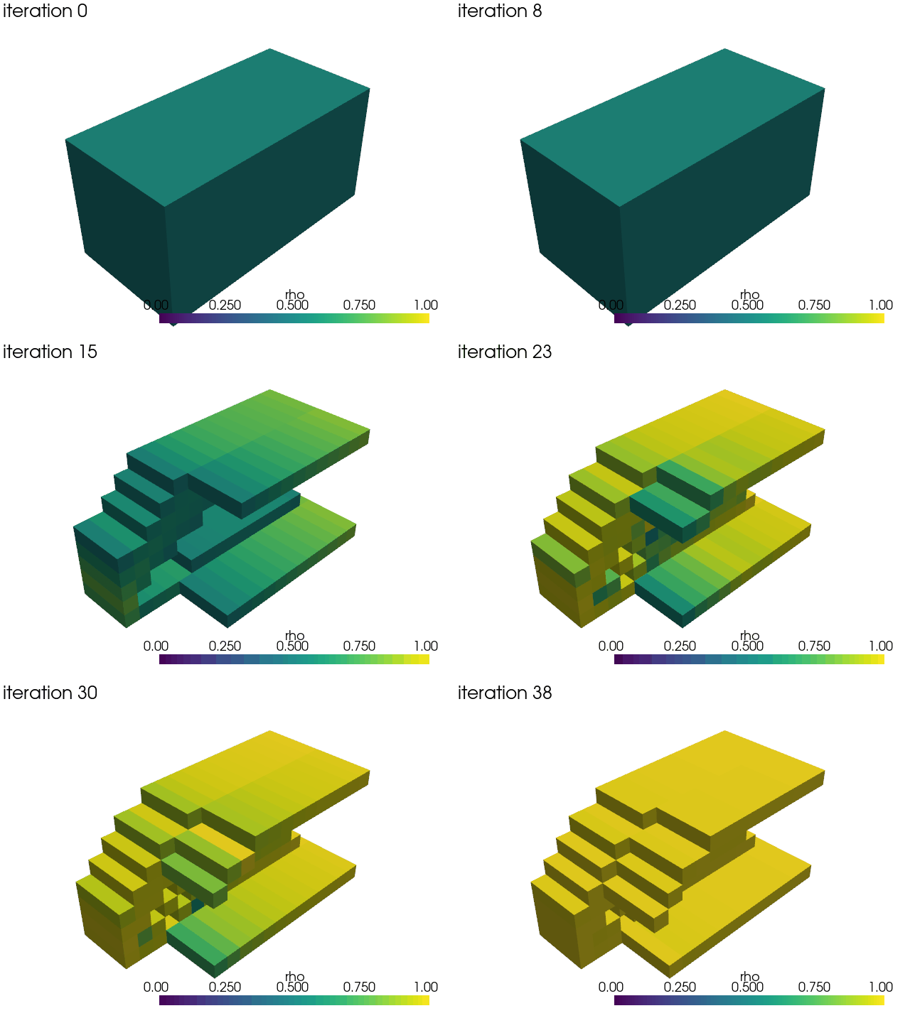
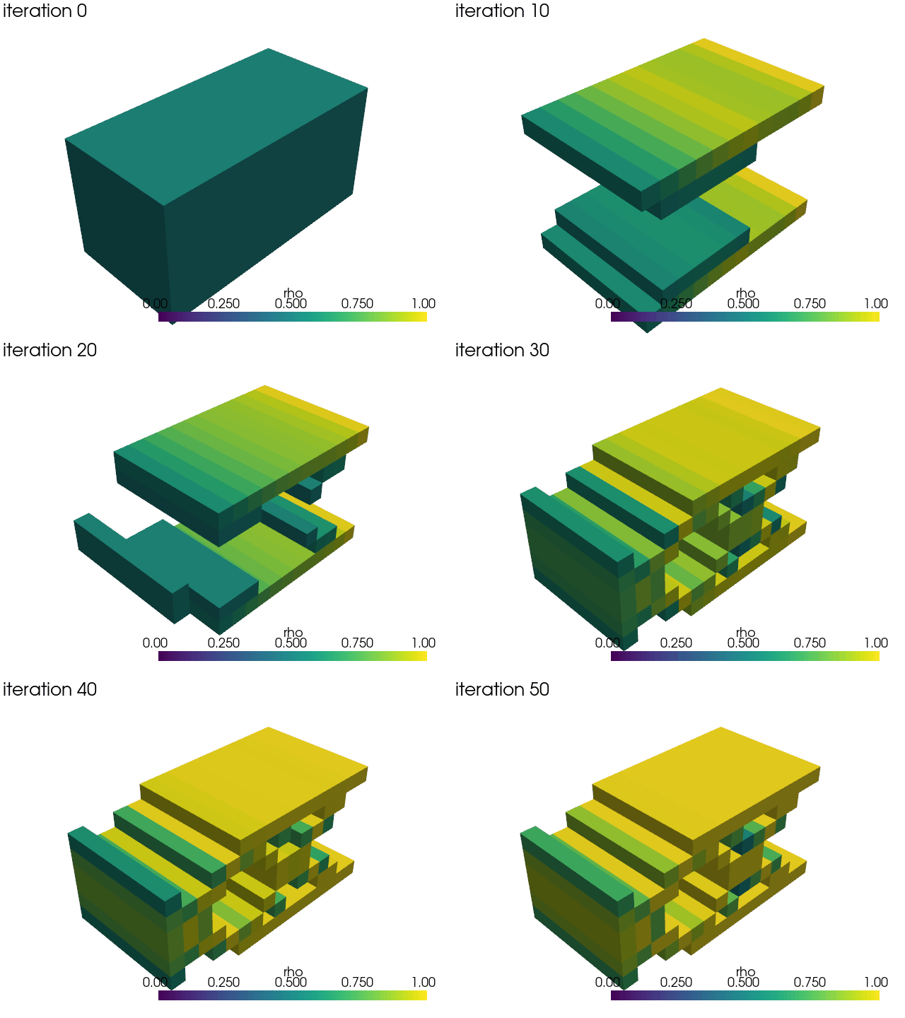
We record the density field once per outer optimizer iteration into a GIF, using the pyvista pattern from dolfinx-tutorial/chapter2/amr.py. Since a SIMP density field lives in a ("DG", 0) space, its dof array maps 1-to-1 onto the local cell numbering, so it can be attached directly as cell_data on a grid built from the mesh itself (not from the function space). We also record the compliance (not the volume-penalized objective) at each iteration.

scipy.optimize.minimize() reports only the penalized objective (intermediate_result.fun), so the pure compliance is recovered arithmetically: since every cell of this structured box mesh has equal volume, the volume fraction is exactly is the mean of rho, so compliance = fun - penalty_weight*(vol_frac - v_frac)**2 recovers it with no extra PDE solve.

def make_iteration_tracker(
    msh: dolfinx.mesh.Mesh, rho: dolfinx_adjoint.Function, gif_path: str, initial_compliance: float
):
    """Return (plotter, callback, compliance_history) tracking one optimizer run."""
    # One frame per outer iteration is embedded in the rendered page, so the frames are
    # kept well below the default 1024x768 to keep the page a reasonable size.
    plotter = pyvista.Plotter(off_screen=True, window_size=PLOT_WINDOW_SIZE)
    plotter.open_gif(gif_path, fps=5)
    compliance_history = [initial_compliance]
    frame_index = itertools.count()

    def write_frame():
        grid = pyvista.UnstructuredGrid(*dolfinx.plot.vtk_mesh(msh))
        grid.cell_data["rho"] = rho.x.array
        filtered_grid = grid.threshold(0.5, scalars="rho")
        actor = plotter.add_mesh(filtered_grid, scalars="rho", clim=(0.0, 1.0), cmap="viridis", show_edges=False)
        # Passing `name` replaces the previous label rather than stacking one text actor
        # per frame, so only the mesh actor has to be removed again below.
        plotter.add_text(f"iteration {next(frame_index)}", font_size=10, name="iteration")
        plotter.view_isometric()
        plotter.write_frame()
        plotter.remove_actor(actor)

    def callback(intermediate_result):
        rho.x.array[:] = intermediate_result.x
        rho.x.scatter_forward()
        write_frame()
        num_dofs_local = rho.function_space.dofmap.index_map.size_local
        local_vol_frac = np.sum(rho.x.array[:num_dofs_local])
        vol = rho.function_space.mesh.comm.allreduce(local_vol_frac, op=MPI.SUM)
        vol_frac = vol / rho.function_space.dofmap.index_map.size_global
        compliance_history.append(intermediate_result.fun - penalty_weight * (vol_frac - v_frac) ** 2)

    write_frame()  # record the initial, uniform density as frame 0
    return plotter, callback, compliance_history

Forward model, gradient verification and optimization

run_topopt builds the forward model once (SIMP weak form, linear solve, compliance

• volume-penalty objective), verifies the resulting adjoint gradient and Hessian with 0th/1st/2nd-order Taylor tests, times a single tape recompute and a single adjoint solve.

def run_topopt(
    corner_load: bool, nx: int = 16, ny: int = 2, nz: int = 8
) -> tuple[
    pyadjoint.ReducedFunctional, dolfinx_adjoint.LinearProblem, pyadjoint.AdjFloat, dolfinx_adjoint.Function, dict
]:
    print(f"\n=== Running topology optimization: {corner_load=} ===")

    pyadjoint.get_working_tape().clear_tape()

    msh, facet_tags, traction = build_mesh_and_bcs(nx, ny, nz, corner_load)
    ds = ufl.Measure("ds", domain=msh, subdomain_data=facet_tags)
    fdim = msh.topology.dim - 1

    # ### Function spaces and control
    V = dolfinx.fem.functionspace(msh, ("Lagrange", 1, (3,)))  # displacement
    Q = dolfinx.fem.functionspace(msh, ("DG", 0))  # density

    rho = dolfinx_adjoint.Function(Q, name="Density")
    rho.x.array[:] = v_frac
    rho.x.scatter_forward()

    uh = dolfinx_adjoint.Function(V, name="Displacement")

    # ### SIMP material law and weak form
    E_min = x_min * E_max
    E = E_min + (E_max - E_min) * rho**penal
    lam = E * nu / ((1 + nu) * (1 - 2 * nu))
    mu = E / (2 * (1 + nu))

    def eps(w):
        return ufl.sym(ufl.grad(w))

    def sigma(w):
        return lam * ufl.tr(eps(w)) * ufl.Identity(3) + 2 * mu * eps(w)

    u, v = ufl.TrialFunction(V), ufl.TestFunction(V)
    a = ufl.inner(sigma(u), eps(v)) * ufl.dx
    t = dolfinx.fem.Constant(msh, traction)
    L = ufl.inner(t, v) * ds(1)

    # ### Dirichlet BC and forward solve (once)
    bdofs = dolfinx.fem.locate_dofs_topological(V, fdim, facet_tags.find(2))
    bc = dolfinx.fem.dirichletbc(np.zeros(3, dtype=dolfinx.default_scalar_type), bdofs, V)

    petsc_options = {
        "ksp_type": "preonly",
        "pc_type": "lu",
        "pc_factor_mat_solver_type": "mumps",
        "ksp_error_if_not_converged": True,
    }
    problem = dolfinx_adjoint.LinearProblem(
        a,
        L,
        u=uh,
        bcs=[bc],
        petsc_options=petsc_options,
        adjoint_petsc_options=petsc_options,
        tlm_petsc_options=petsc_options,
    )

    t_forward_start = time.perf_counter()
    problem.solve()
    forward_time = time.perf_counter() - t_forward_start
    print(f"[{corner_load=}] initial forward solve: {forward_time:.4e} s")

    # ### Objective: compliance + volume-fraction penalty
    compliance = dolfinx_adjoint.assemble_scalar(ufl.action(L, uh))
    vol_frac = dolfinx_adjoint.assemble_scalar(rho * ufl.dx) / (Lx * Ly * Lz)
    J = compliance + penalty_weight * (vol_frac - v_frac) ** 2

    control = pyadjoint.Control(rho)
    Jhat = pyadjoint.ReducedFunctional(J, control)

    # ### Gradient and Hessian verification: 0th, 1st and 2nd-order Taylor tests
    with pyadjoint.stop_annotating():
        h = dolfinx_adjoint.Function(Q)
        rng = np.random.default_rng(seed=42)
        h.x.array[:] = rng.standard_normal(len(h.x.array))
        h.x.scatter_forward()

        rate0 = pyadjoint.taylor_test(Jhat, rho, h, dJdm=0)
        print(f"[{corner_load=}] 0th-order Taylor rate (expect ~1): {rate0:.4f}")
        rate1 = pyadjoint.taylor_test(Jhat, rho, h)
        print(f"[{corner_load=}] 1st-order Taylor rate (expect ~2): {rate1:.4f}")

        Jhat(rho)
        dJdm = Jhat.derivative()._ad_dot(h)
        dHddu = Jhat.hessian(h)._ad_dot(h)
        rate2 = pyadjoint.taylor_test(Jhat, rho, h, dJdm=dJdm, Hm=dHddu)
        print(f"[{corner_load=}] 2nd-order Taylor rate (expect ~3): {rate2:.4f}")

    # ### Cost of one recompute vs. one adjoint solve
    #
    # Mirrors the forward-vs-VJP cost split Mosaic itself tracks separately
    # (`cost/spatial_cost` vs `cost/vjp_cost`).
    t_recompute_start = time.perf_counter()
    Jhat(rho)
    recompute_time = time.perf_counter() - t_recompute_start
    print(f"[{corner_load=}] one tape recompute (Jhat(rho)): {recompute_time:.4e} s")

    t_derivative_start = time.perf_counter()
    Jhat.derivative()
    derivative_time = time.perf_counter() - t_derivative_start
    print(f"[{corner_load=}] one adjoint solve (Jhat.derivative()): {derivative_time:.4e} s")
    timings = {"recompute_time": recompute_time, "derivative_time": derivative_time, "forward_time": forward_time}
    return Jhat, problem, compliance, rho, timings

Bound- and curvature-aware optimization

scipy.optimize.minimize(method="trust-constr") is the scipy method that accepts both bounds= and a Hessian-vector product (hessp=); pyadjoint.minimize’s convenience wrapper only wires hessp automatically for method="Newton-CG" (which has no bounds support), so we drive scipy.optimize.minimize directly from a pyadjoint.reduced_functional_numpy.ReducedFunctionalNumPy — the same public class pyadjoint.minimize itself wraps every call in.

def optimize(
    rho: dolfinx_adjoint.Function,
    Jhat: pyadjoint.ReducedFunctional,
    problem: dolfinx_adjoint.LinearProblem,
    compliance: pyadjoint.AdjFloat,
    corner_load: bool,
):
    case_name = "corner_load" if corner_load else "full_face_load"
    gif_path = f"topopt_{case_name}.gif"
    msh = rho.function_space.mesh
    plotter, callback, compliance_history = make_iteration_tracker(msh, rho, gif_path, float(compliance))

    rf_np = pyadjoint.reduced_functional_numpy.ReducedFunctionalNumPy(Jhat)
    m0 = rf_np.get_controls()

    t_optim_start = time.perf_counter()
    res = scipy.optimize.minimize(
        fun=rf_np.__call__,
        x0=m0,
        jac=lambda m: rf_np.derivative(),
        hessp=lambda m, p: rf_np.hessian(p),
        method="trust-constr",
        bounds=scipy.optimize.Bounds(x_min, 1.0),
        callback=callback,
        options={"maxiter": 200, "verbose": 2},
    )
    optim_time = time.perf_counter() - t_optim_start
    print(f"[{case_name}] trust-constr optimization: {optim_time:.4e} s over {res.nit} iterations")

    rho_opt = rf_np.set_controls(res.x)[0]
    rho.x.array[:] = rho_opt.x.array
    rho.x.scatter_forward()
    problem.solve(annotate=False)
    plotter.close()

    # Final compliance/volume fraction as plain floats.
    uh = problem.u
    L = problem._rhs
    final_compliance = dolfinx_adjoint.assemble_scalar(ufl.action(L, uh), annotate=False)
    final_vol_frac = dolfinx_adjoint.assemble_scalar(rho * ufl.dx, annotate=False) / (Lx * Ly * Lz)

    # The converged density field.
    grid = pyvista.UnstructuredGrid(*dolfinx.plot.vtk_mesh(msh))
    grid.cell_data["rho"] = rho.x.array
    filtered_grid = grid.threshold(0.5, scalars="rho")
    final_plotter = pyvista.Plotter(off_screen=pyvista.OFF_SCREEN, window_size=PLOT_WINDOW_SIZE)
    final_plotter.add_text(case_name, font_size=10)
    final_plotter.add_mesh(filtered_grid, scalars="rho", clim=(0.0, 1.0), cmap="viridis", show_edges=False)
    final_plotter.view_isometric()

    return {
        "case": case_name,
        "compliance": float(final_compliance),
        "vol_frac": float(final_vol_frac),
        "n_iterations": int(res.nit),
        "optim_time": optim_time,
        "compliance_history": compliance_history,
        "gif_path": gif_path,
        "plotter": final_plotter,
    }

Running both load cases

Mosaic’s canonical optimization/topopt run uses corner_load=True; we additionally run the uniform full-face load for comparison. We use the settings from the benchmark website to enable a suitable runtime for the optimization. For other settings, see [RZH26].

trust-constr logs a row per iteration, so this cell carries the output_scroll tag: the log is rendered as a scroll box instead of several screens of text.

results = []
for corner_load in [True, False]:
    Jhat, problem, compliance, rho, timings = run_topopt(corner_load, nx=16, ny=2, nz=8)
    result = optimize(rho, Jhat, problem, compliance, corner_load)
    result.update(timings)
    results.append(result)

=== Running topology optimization: corner_load=True ===

[corner_load=True] initial forward solve: 2.0989e-02 s

Running Taylor test
Computed residuals: [6.53515011999643e-05, 2.9691899758083236e-05, 1.4102626766038587e-05, 6.8658060172104365e-06]
Computed convergence rates: [1.1381509734598056, 1.0741054981902485, 1.038462903279684]
[corner_load=True] 0th-order Taylor rate (expect ~1): 1.0385

Running Taylor test
Computed residuals: [1.1907407594145677e-05, 2.969852955173927e-06, 7.416033645839324e-07, 1.8529431648310934e-07]
Computed convergence rates: [2.0033959464245177, 2.001671806903951, 2.0008291589675653]
[corner_load=True] 1st-order Taylor rate (expect ~2): 2.0008

Running Taylor test
Computed residuals: [5.534755899028915e-08, 6.837946385080118e-09, 8.496123867206541e-10, 1.0587843380641044e-10]
Computed convergence rates: [3.016884674749586, 3.0086864061075156, 3.0043960405063257]
[corner_load=True] 2nd-order Taylor rate (expect ~3): 3.0044
[corner_load=True] one tape recompute (Jhat(rho)): 1.9137e-02 s
[corner_load=True] one adjoint solve (Jhat.derivative()): 2.8962e-02 s

| niter |f evals|CG iter|  obj func   |tr radius |   opt    |  c viol  |
|-------|-------|-------|-------------|----------|----------|----------|
|   1   |   1   |   0   | +4.8853e-03 | 1.00e+00 | 3.42e-04 | 0.00e+00 |

|   2   |   2   |   2   | +4.8597e-03 | 5.60e+00 | 1.64e-05 | 0.00e+00 |

|   3   |   3   |   4   | +4.8688e-03 | 3.14e+01 | 1.89e-05 | 0.00e+00 |

|   4   |   4   |   5   | +4.8764e-03 | 3.14e+01 | 1.68e-05 | 0.00e+00 |

|   5   |   4   |   5   | +4.8764e-03 | 1.57e+02 | 8.03e-05 | 0.00e+00 |

|   6   |   4   |   5   | +4.8764e-03 | 7.84e+02 | 9.31e-05 | 0.00e+00 |

|   7   |   4   |   5   | +4.8764e-03 | 3.92e+03 | 9.56e-05 | 0.00e+00 |

|   8   |   4   |   5   | +4.8764e-03 | 1.96e+04 | 9.61e-05 | 0.00e+00 |

|   9   |   5   |   8   | +3.7326e-03 | 1.96e+04 | 4.06e-05 | 0.00e+00 |

|  10   |   5   |   8   | +3.7326e-03 | 9.80e+04 | 5.10e-05 | 0.00e+00 |

|  11   |   6   |  12   | +2.6355e-03 | 9.80e+04 | 2.25e-05 | 0.00e+00 |

|  12   |   7   |  14   | +2.5999e-03 | 9.80e+04 | 2.82e-06 | 0.00e+00 |

|  13   |   7   |  14   | +2.5999e-03 | 4.90e+05 | 6.31e-06 | 0.00e+00 |

|  14   |   8   |  20   | +2.5999e-03 | 4.90e+04 | 6.31e-06 | 0.00e+00 |

|  15   |  10   |  22   | +2.5999e-03 | 4.90e+03 | 6.31e-06 | 0.00e+00 |

|  16   |  11   |  26   | +1.7576e-03 | 4.90e+03 | 1.47e-06 | 0.00e+00 |

|  17   |  12   |  30   | +1.7404e-03 | 4.90e+03 | 3.59e-07 | 0.00e+00 |

|  18   |  12   |  30   | +1.7404e-03 | 2.45e+04 | 9.25e-07 | 0.00e+00 |

|  19   |  13   |  34   | +1.3390e-03 | 2.45e+04 | 1.13e-06 | 0.00e+00 |

|  20   |  14   |  39   | +1.2402e-03 | 2.45e+04 | 2.46e-06 | 0.00e+00 |

|  21   |  15   |  44   | +1.2402e-03 | 2.45e+03 | 2.46e-06 | 0.00e+00 |

|  22   |  16   |  51   | +1.2339e-03 | 2.45e+03 | 4.80e-07 | 0.00e+00 |

|  23   |  18   |  55   | +1.2339e-03 | 2.45e+02 | 4.80e-07 | 0.00e+00 |

|  24   |  19   |  58   | +1.2285e-03 | 2.45e+02 | 8.02e-07 | 0.00e+00 |

|  25   |  20   |  62   | +1.2285e-03 | 2.45e+01 | 8.02e-07 | 0.00e+00 |

|  26   |  21   |  65   | +1.2251e-03 | 2.45e+01 | 6.27e-07 | 0.00e+00 |

|  27   |  21   |  65   | +1.2251e-03 | 1.23e+02 | 6.19e-07 | 0.00e+00 |

|  28   |  22   |  69   | +1.2251e-03 | 1.23e+01 | 6.19e-07 | 0.00e+00 |

|  29   |  24   |  70   | +1.2251e-03 | 6.13e+00 | 6.19e-07 | 0.00e+00 |

|  30   |  25   |  72   | +1.1274e-03 | 4.29e+01 | 1.46e-06 | 0.00e+00 |

|  31   |  26   |  74   | +1.0898e-03 | 4.29e+01 | 3.36e-07 | 0.00e+00 |

|  32   |  27   |  76   | +1.0595e-03 | 4.29e+01 | 8.71e-07 | 0.00e+00 |

|  33   |  28   |  77   | +1.0594e-03 | 4.29e+01 | 2.40e-07 | 0.00e+00 |

|  34   |  29   |  80   | +1.0594e-03 | 4.29e+00 | 2.40e-07 | 0.00e+00 |

|  35   |  30   |  85   | +1.0416e-03 | 8.58e+00 | 2.24e-07 | 0.00e+00 |

|  36   |  31   |  87   | +1.0407e-03 | 8.58e+00 | 5.53e-08 | 0.00e+00 |

|  37   |  31   |  87   | +1.0407e-03 | 4.29e+01 | 2.63e-08 | 0.00e+00 |

|  38   |  32   |  89   | +1.0123e-03 | 5.64e+01 | 9.18e-09 | 0.00e+00 |

`gtol` termination condition is satisfied.
Number of iterations: 38, function evaluations: 32, CG iterations: 89, optimality: 9.18e-09, constraint violation: 0.00e+00, execution time: 2.6e+01 s.
[corner_load] trust-constr optimization: 2.6398e+01 s over 38 iterations

=== Running topology optimization: corner_load=False ===
[corner_load=False] initial forward solve: 1.9667e-02 s
Running Taylor test
Computed residuals: [4.951646264201182e-05, 2.190901529489954e-05, 1.0244055081052965e-05, 4.944641280442592e-06]
Computed convergence rates: [1.1763836113915083, 1.096737728299671, 1.0508491487649372]
[corner_load=False] 0th-order Taylor rate (expect ~1): 1.0508
Running Taylor test

Computed residuals: [1.1377227039708292e-05, 2.839397493747774e-06, 7.092461804770821e-07, 1.7723683015465102e-07]
Computed convergence rates: [2.002492239362394, 2.0012264481301476, 2.0006080462811267]
[corner_load=False] 1st-order Taylor rate (expect ~2): 2.0006
Running Taylor test

Computed residuals: [3.882187740564578e-08, 4.796203172112258e-09, 5.958578331667515e-10, 7.424949367217055e-11]
Computed convergence rates: [3.0169052085058103, 3.0088527125434275, 3.004515063517032]
[corner_load=False] 2nd-order Taylor rate (expect ~3): 3.0045
[corner_load=False] one tape recompute (Jhat(rho)): 1.9417e-02 s
[corner_load=False] one adjoint solve (Jhat.derivative()): 2.8600e-02 s

| niter |f evals|CG iter|  obj func   |tr radius |   opt    |  c viol  |
|-------|-------|-------|-------------|----------|----------|----------|
|   1   |   1   |   0   | +4.1199e-03 | 1.00e+00 | 1.87e-04 | 0.00e+00 |

|   2   |   2   |   2   | +4.1016e-03 | 5.60e+00 | 7.11e-06 | 0.00e+00 |

|   3   |   3   |   4   | +4.1082e-03 | 3.14e+01 | 1.10e-05 | 0.00e+00 |

|   4   |   4   |   5   | +4.1141e-03 | 3.14e+01 | 1.19e-05 | 0.00e+00 |

|   5   |   4   |   5   | +4.1141e-03 | 1.57e+02 | 3.93e-05 | 0.00e+00 |

|   6   |   4   |   5   | +4.1141e-03 | 7.84e+02 | 4.48e-05 | 0.00e+00 |

|   7   |   4   |   5   | +4.1141e-03 | 3.92e+03 | 4.59e-05 | 0.00e+00 |

|   8   |   4   |   5   | +4.1141e-03 | 1.96e+04 | 4.61e-05 | 0.00e+00 |

|   9   |   4   |   5   | +4.1141e-03 | 9.80e+04 | 4.62e-05 | 0.00e+00 |

|  10   |   5   |   9   | +1.9781e-03 | 9.80e+04 | 1.08e-05 | 0.00e+00 |

|  11   |   6   |  14   | +1.9781e-03 | 9.80e+03 | 1.08e-05 | 0.00e+00 |

|  12   |   8   |  18   | +1.9781e-03 | 9.80e+02 | 1.08e-05 | 0.00e+00 |

|  13   |   9   |  24   | +1.9781e-03 | 9.80e+01 | 1.08e-05 | 0.00e+00 |

|  14   |  10   |  30   | +1.9781e-03 | 9.80e+00 | 1.08e-05 | 0.00e+00 |

|  15   |  11   |  34   | +2.3292e-03 | 1.96e+01 | 9.46e-06 | 0.00e+00 |

|  16   |  11   |  34   | +2.3292e-03 | 9.80e+01 | 9.33e-06 | 0.00e+00 |

|  17   |  12   |  37   | +1.9883e-03 | 9.80e+01 | 4.78e-06 | 0.00e+00 |

|  18   |  13   |  45   | +1.9883e-03 | 9.80e+00 | 4.78e-06 | 0.00e+00 |

|  19   |  15   |  47   | +1.9883e-03 | 9.80e-01 | 4.78e-06 | 0.00e+00 |

|  20   |  16   |  49   | +1.9489e-03 | 1.96e+00 | 1.82e-06 | 0.00e+00 |

|  21   |  16   |  49   | +1.9489e-03 | 9.80e+00 | 2.50e-06 | 0.00e+00 |

|  22   |  17   |  52   | +1.6086e-03 | 5.09e+01 | 1.35e-06 | 0.00e+00 |

|  23   |  18   |  55   | +1.4107e-03 | 5.19e+01 | 3.68e-06 | 0.00e+00 |

|  24   |  19   |  63   | +1.4107e-03 | 5.19e+00 | 3.68e-06 | 0.00e+00 |

|  25   |  20   |  66   | +1.2919e-03 | 1.04e+01 | 9.27e-07 | 0.00e+00 |

|  26   |  21   |  71   | +1.1918e-03 | 1.73e+01 | 6.82e-07 | 0.00e+00 |

|  27   |  22   |  76   | +1.1918e-03 | 1.73e+00 | 6.82e-07 | 0.00e+00 |

|  28   |  23   |  78   | +1.1931e-03 | 3.46e+00 | 1.10e-06 | 0.00e+00 |

|  29   |  24   |  81   | +1.2063e-03 | 6.92e+00 | 2.06e-06 | 0.00e+00 |

|  30   |  25   |  83   | +1.2010e-03 | 6.92e+00 | 9.64e-07 | 0.00e+00 |

|  31   |  26   |  87   | +1.2191e-03 | 1.38e+01 | 1.26e-06 | 0.00e+00 |

|  32   |  27   |  93   | +1.2185e-03 | 2.77e+01 | 4.52e-06 | 0.00e+00 |

|  33   |  28   |  94   | +1.2181e-03 | 2.77e+01 | 2.53e-07 | 0.00e+00 |

|  34   |  28   |  94   | +1.2181e-03 | 1.38e+02 | 3.32e-07 | 0.00e+00 |

|  35   |  29   |  98   | +1.0814e-03 | 1.38e+02 | 2.19e-07 | 0.00e+00 |

|  36   |  30   |  102  | +1.0571e-03 | 1.38e+02 | 2.34e-07 | 0.00e+00 |

|  37   |  31   |  119  | +1.0571e-03 | 1.38e+01 | 2.34e-07 | 0.00e+00 |

|  38   |  33   |  122  | +1.0571e-03 | 2.04e+00 | 2.34e-07 | 0.00e+00 |

|  39   |  35   |  124  | +1.0571e-03 | 1.02e+00 | 2.34e-07 | 0.00e+00 |

|  40   |  36   |  129  | +1.0569e-03 | 2.04e+00 | 3.25e-07 | 0.00e+00 |

|  41   |  37   |  133  | +1.0578e-03 | 4.09e+00 | 9.93e-08 | 0.00e+00 |

|  42   |  38   |  138  | +1.0587e-03 | 8.18e+00 | 1.46e-07 | 0.00e+00 |

|  43   |  39   |  147  | +1.0603e-03 | 1.64e+01 | 6.32e-08 | 0.00e+00 |

|  44   |  39   |  147  | +1.0603e-03 | 8.18e+01 | 7.52e-08 | 0.00e+00 |

|  45   |  40   |  154  | +1.0240e-03 | 8.18e+01 | 7.13e-08 | 0.00e+00 |

|  46   |  41   |  164  | +1.0240e-03 | 8.18e+00 | 7.13e-08 | 0.00e+00 |

|  47   |  42   |  174  | +1.0218e-03 | 8.18e+00 | 1.91e-07 | 0.00e+00 |

|  48   |  43   |  179  | +1.0151e-03 | 2.52e+01 | 1.44e-07 | 0.00e+00 |

|  49   |  44   |  183  | +1.0145e-03 | 2.52e+01 | 4.08e-08 | 0.00e+00 |

|  50   |  45   |  202  | +1.0131e-03 | 2.52e+01 | 6.76e-09 | 0.00e+00 |

`gtol` termination condition is satisfied.
Number of iterations: 50, function evaluations: 45, CG iterations: 202, optimality: 6.76e-09, constraint violation: 0.00e+00, execution time: 4.2e+01 s.
[full_face_load] trust-constr optimization: 4.2599e+01 s over 50 iterations

Optimised designs

The per-iteration density animation and the converged design for each load case.

for result in results:
    display(Markdown(f"**{result['case']}**"))
    display(Image(filename=result["gif_path"]))
    if pyvista.OFF_SCREEN:
        result["plotter"].screenshot(f"topopt_{result['case']}_final.png")
    else:
        result["plotter"].show()

corner_load

full_face_load

Summary

summary = pandas.DataFrame(results).set_index("case")
print("\n=== Summary ===")
print(summary.drop(columns=["compliance_history", "gif_path", "plotter"]))

=== Summary ===
                compliance  vol_frac  n_iterations  optim_time  \
case                                                             
corner_load       0.001012  0.500004            38   26.397994   
full_face_load    0.001013  0.500021            50   42.598609   

                recompute_time  derivative_time  forward_time  
case                                                           
corner_load           0.019137         0.028962      0.020989  
full_face_load        0.019417         0.028600      0.019667  

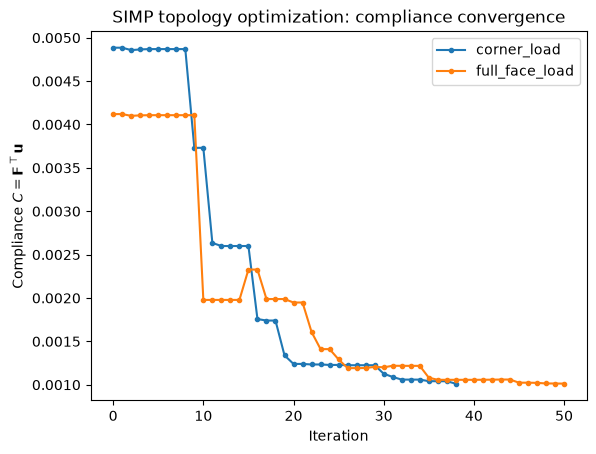
Compliance convergence

A compliance-vs-iteration plot, as shown on Mosaic’s own results page.

fig, ax = plt.subplots()
for result in results:
    ax.plot(result["compliance_history"], marker="o", markersize=3, label=result["case"])
ax.set_xlabel("Iteration")
ax.set_ylabel("Compliance $C = \\mathbf{F}^\\top \\mathbf{u}$")
ax.set_title("SIMP topology optimization: compliance convergence")
ax.legend()
fig.savefig("topopt_compliance_convergence.png", dpi=150, bbox_inches="tight")
plt.show()

References

[RZH26]

Andrin Rehmann, Heiko Zimmermann, and Dion Häfner. Mosaic: a benchmark suite for differentiable physics solvers. 2026. URL: https://arxiv.org/abs/2606.27895, arXiv:2606.27895.